| Japanese | English |
Design Specification
1. Noise Cancelling Algorithm[1]1-1. Specter Subtraction Method (SS Method)
1-2. MAP method using Variable Speech Distribution
1-2-1. MAP Estimate Method
1-2-2. Speech spectrum distribution proposed by T.Lotter and P.Vary
1-2-3. Variable Speech Distribution
2. Implementation of the Noise Cancelling System
2-1.Separating into the Hardware and the Software
2-1-1.Features of the HW and the SW
2-1-2. Feature of Noise Cancelling System
2-1-3. Architecture
2-2. Hardware
2-2-1. Processing flow
2-2-2. Circuit structure
2-2-3. HW timing
2-3. Software
2-3-1. Source code
2-3-2. Flow chart
3. Development Environment
3-1. Hardware Design Process
3-1-1. Design Hardware Logic
3-1-2. Manual of Xilinx ISE and EDK
3-2. Software design process
4. Contest Design Target
5. SPEED and AREA
6. References
7. Download
17th LSI Design Contests・in Okinawa Design Specification - 1
1. Noise Cancelling Algorithm
To remove noise, there are some methods are suggested such as Microphone Array Method which is used several microphones and method using adaptive filtering to presume unknown pathway. In this simulation, the Noise Cancelling System by using Specter Subtraction Method (SS Method) which removes the noise in frequency domain is targeted.
The difference from last year is that we introduce other efficient techniques described in Sec. 1-2.
1-1. Specter Subtraction Method (SS Method)
In this section, the Noise Cancelling Algorithm is explained. The algorithm removes the noise in frequency domain. A diagram of the Noise Cancelling Algorithm is shown in Figure 1.
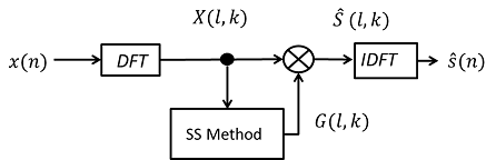
Figure 1
First, the observed signal is assumed to be given by the sum of speech and noise. The observed signal, the speech and the noise at time n are defined as x(n), s(n) and d(n) respectively. Then, the observed signal x(n) is expressed by
when the speech and the noise are uncorrelated.
Next, to remove noise in frequency domain, the Discrete Fourier Transform (DFT) applies the observed signal x(n). After that, the observed signal specter X(l,k) from top to k in l-frame is expressed by
when S(l,k) and D(l,k) denote the speech specter and the noise specter respectively.
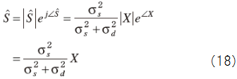
The estimate value of speech ![]() is expressed by the observed signal specter X(l,k) as.
is expressed by the observed signal specter X(l,k) as.
Here, G(l,k) is a specter gain, and the estimate value specter is result of the observed signal specter X(l,k) multiplied by suitable specter gain G(l,k).
The ideal estimate value ![]() is expressed by
is expressed by
By substituting eq.(4) into eq.(3), the ideal specter gain G_opt (l,k) given as.
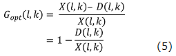
Then, the speech specter X(l,k) is extracted perfectly. However, the noise specter D(l,k) can’t be obtained by only the speech specter X(l,k)’s
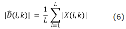
information. Therefore, for SS Method, the noise specter estimate value ![]() can be obtained by using the ‘L’ number of frames in non-speech interval.
can be obtained by using the ‘L’ number of frames in non-speech interval. ![]() is defined as
is defined as
The simulation of the SS method was performed by Scilab. The result is shown in Figure 2. We can download the program (here).
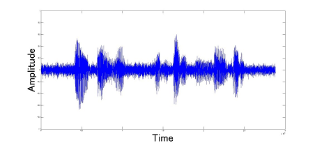
(a)Input Signal
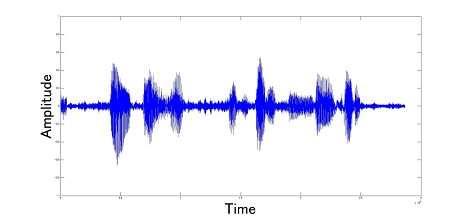
(a)Output Signal
Figure 2
1-2. MAP method using Variable Speech Distribution
This is a new algorithm that we introduce this year. The file related to the algorithm was put in the DL_file_ver3 at here.
1-2-1. MAP Estimate Method
Object
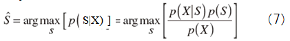

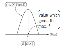
Figure 3
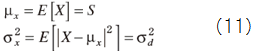
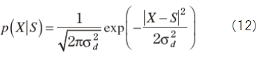
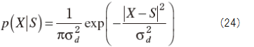
・PDF to S and D
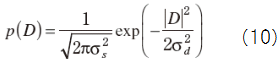
Suppose X=const.+D and no relation between D and S, then
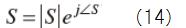
Define ε in order to maximize S as
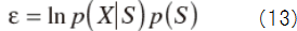
S can be rewritten as
Now we want to get following
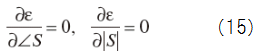
↓
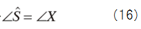
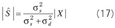
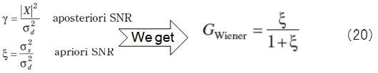
From (16) and (17), we get
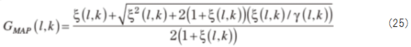
Therefore we get the spectrum gain
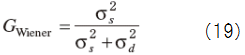
When we difine
・Decision-Directed Mehod
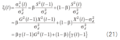
We often choose β=0.98 and γ(l) - 1 should be positive so that

・MAP Method
Most of speech signal follows Rayleigh distribution rather than Gaussian one

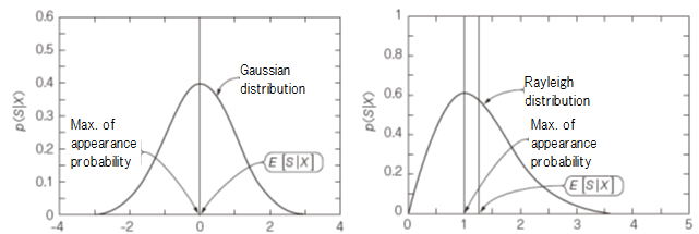
Figure 4
Suppose real and imaginary part of noise are uncorrelated each other with half of variance,
As same manner from (13) to (19), we get the spectrum gain for MAP estimate.
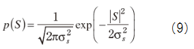
1-2-2. Speech spectrum distribution proposed by T.Lotter and P.Vary
PDF (Probability Density Function) of the speech spectrum that has been proposed by T.Lotter and P.Vary is one of the useful. According to them, the phase spectrum can be expressed approximately by an uniform distribution, the amplitude spectrum is also expressed approximately by the equation (7).
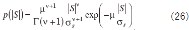
Γ(・) is the gamma function. ν and μ, is a parameter that determines the shape of the distribution. The figure 3 shows the PDF given by equation (26).
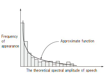
Figure 5
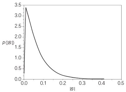
Figure 6
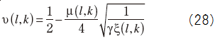
We get the spectrum gain for Lotter/Vary method
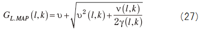
where
MAP estimated value of the phase spectrum and the phase spectrum of the observed signal.
1-2-3. Variable Speech Distribution
We show how to change voice PDF in Figure 5.
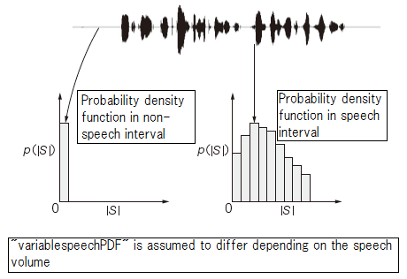
Figure 7
It is called Variable Speech PDF method that we adaptively change the shape of the speech spectrum distribution in the non-speech section and the speech section.
Equation (7) can be approximated to a Rayleigh distribution from exponential distribution by the parameter ν. We show the distribution curve which equation (7) gives on the case of each ν in Figure 6, and we fixed μ to 3.2.
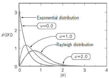
Figure 8
When ν=0.0 Equation (7) match an exponential distribution, and when ν=2.0 (7) is approximated to a Rayleigh distribution. It means that we can approximate to the change of actual speechPDF by changing the value of ν.
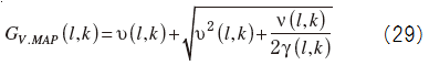
The spectral gain based on the variable speech distribution is obtained by allowing variation in the spectral gain parameter of Lotter/Vary's.
The algorithm for determining ν(l,k) is given by
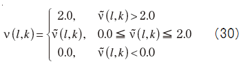
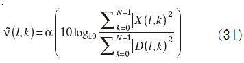
N is the number of FFT spectrum, and α is a parameter for adjusting the size of ν~(l,k).
The simulation of the MAP method was performed by Scilab. The result is shown in Figure 7. You can download the program here.
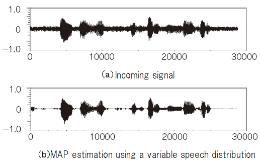
Figure 9
References
[1] T. Lotter, P. Vary ; Speech enhancement by MAP spectral amplitude estimation using a super-Gaussian speech model, EURASIP Journal on Applied Signal Processing, 2005.
[2] A. Kawamura, M. Kurosaki ; 大容量化するマルチメディア・データを転送・保存・活用するために ディジタル音声&画像の圧縮/伸張/加工技術, in H. Ochi, CQ Publishing Co., 2013.